Does a win always reset the payout to 1400?

No. In the stated convention it reduces the level by one. The starting level is required.

Is 24.137931% a universal force-buy threshold?

No. It follows only from the explicit two-round assumptions; it is not a measured CS2 rate.

Does the plant prove an advantage?

No. Conditional cash income does not establish inventory, spending, win probability or an executable price.

MR12 economy: loss counters and conditional round models

Under a twelve-round half, one round is 1/12 of the schedule, or 8.333333%; under fifteen rounds it is 6.666667%. That count does not say how much a round changes map-win probability. The examples here separate format, cash state and a conditional forecast. They do not document bookmaker errors or a measured profitable second-round strategy.

The cash convention follows the displayed assumptions of the CS2 simulator: read the current loss level before updating it. Map rates and buy-tier probabilities are assumptions, not calibrated observations. Check the event configuration, cash, retained equipment and information time before applying any branch.

Why MR12 Amplified Round Leverage

A specified three-round recovery occupies 3/12 = 25% of an MR12 half and 3/15 = 20% of an MR15 half. This compares an assumed duration, not a universal recovery law. Spending, saved weapons, other income and outcomes can change the duration. A cash shortage does not force three lost rounds or determine a handicap.

MR12: 1/12 = 8.333333%; 3/12 = 25%
MR15: 1/15 = 6.666667%; 3/15 = 20%
(1/12)/(1/15) - 1 = 25% relative change in round share
This is a count comparison, not a map-win probability.

The Loss Bonus Ladder, Decoded

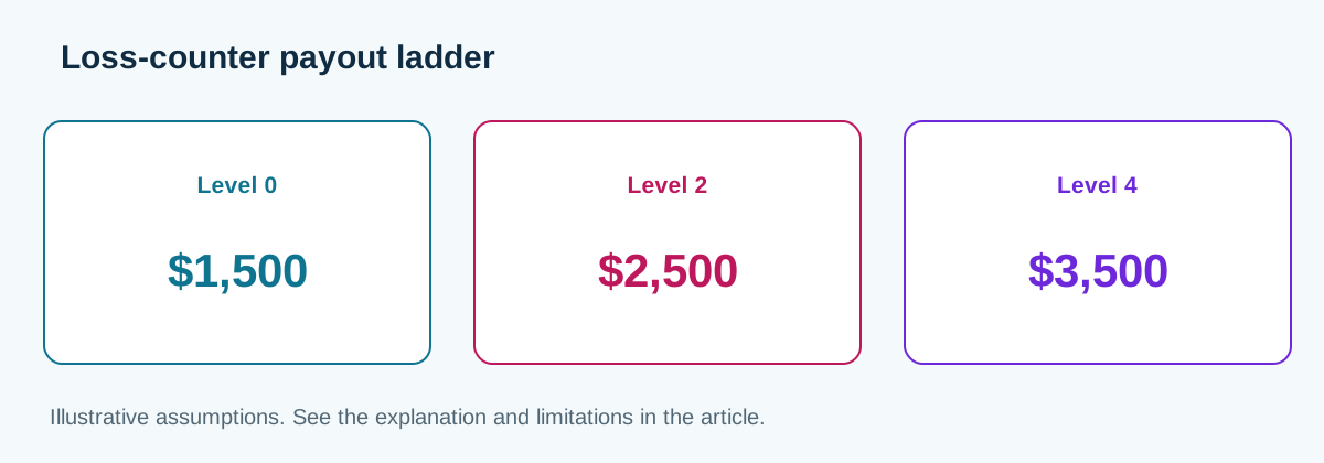
In this eligible-loss cash model, L=0..4 selects payouts 1400, 1900, 2400, 2900 and 3400. A loss pays the current level and then increments it, capped at four. A win reduces the level by one rung, never below zero. This is not simply a consecutive-loss count, and the payout is not the entire next balance.

At the model half-start, L=1. Losing the opening round therefore pays 1900. Winning it leaves L=0, so a following loss pays 1400. Confirm the event settings rather than transferring this initial state to every mid-half example or overtime.

Assume an opening loss at L=1, another loss with zero spending, no other income and no cap effect. The two payouts sum to 1900 + 2400 = 4300. With 100 retained cash the balance is 4400. That does not prove a particular rifle purchase: equipment and purchase decisions still need their own inputs.

Loss Streak Resetting Mechanics: The One-Rung Decrement

Starting at L=4, a win leaves L=3 and the next eligible loss pays 2900. Two wins instead leave L=2 and a subsequent loss pays 2400. Starting at L=2, the same two wins leave L=0 and the payout is 1400. Always preserve the initial level; score alone cannot reconstruct it.

C_next = C_before - spending + eligible income
L_after_loss = min(4, L_before + 1)
L_after_win = max(0, L_before - 1)
C=4800, spending=4700, L=1, loss: C_next=2000
C=2300, spending=2200, L=2, loss: C_next=2500
Same last example + assumed plant income 800: C_next=3300

Break-Even Probability of Second-Round Force Buys

Compare the expected number of rounds in two explicitly assumed plans. Let saving win round two with probability 0.05 and have unconditional round-three win probability 0.45. Under forcing, let the round-three conditional chances be 0.60 after winning and 0.15 after losing. These are illustrative inputs, not measured conversion rates.

E_save = 0.05 + 0.45 = 0.50
E_force = p + p*0.60 + (1-p)*0.15 = 0.15 + 1.45p
p_break_even = (0.50-0.15)/1.45 = 7/29 = 24.137931%
p=0.40 => E_force=0.73 rounds
These are expected round counts, not monetary EV.

The $800 Bomb Plant Dynamic

In the stated model, an eligible plant-loss bonus of 800 is added separately. At half-start L=1, 1900 + 800 = 2700 before other adjustments; with 100 unspent cash it becomes 2800. A balance alone does not establish a buy tier or round-win probability. Check actual inventory and spending rather than inferring an armored loadout from the plant.

The Double Eco Pitfall in MR12

For a hypothetical binomial count, assume twelve independent rounds with constant win chance 0.45. The expected count is 5.4; the probabilities of at most four and at most three wins are 30.443200% and 13.446807%. This is not a fitted CS2 half model: sides and economy can make probabilities unequal and dependent.

Now explicitly fix three rounds as losses and leave nine independent chances at 0.45. The expected total is 4.05; at most four wins has probability 62.142095%, at most three 36.138460%. This conditions on losses. It does not prove that choosing an eco forces those losses, predicts an Under, or makes the opponent profitable.

P(X<=k) = sum(C(n,j)*0.45^j*0.55^(n-j), j=0..k)
n=12: E[X]=5.40
n=9: E[X]=4.05
Independence and constant probability are assumed.

Live Tracking Workflow

Keep separate records for observed cash, initial counter, retained equipment, assumed spending, forecast and accepted quote. If a cash prediction fails, check inputs before changing win probabilities. A correct balance is only a state check; it does not validate a conversion rate. Preserve forecasts before results and evaluate later comparable rounds, including losses and passed decisions.

Model record fields:
map / half / round / side / source time
L_before / cash_before / retained equipment
spending / eligible income / round outcome
L_after / cash_after / forecast revision
market / requested price / accepted price / status

Expected rounds and a bet return answer different questions. Suppose the next-round quote is an invented 3.80. Its break-even probability is 1/3.80 = 26.315789%, regardless of the two-round planning threshold 24.137931%. Choosing a buy that maximizes expected rounds does not establish that any offered wager has positive expectation. Compare the exact event and accepted price after forming a defensible probability, rather than inserting the planning threshold as a team forecast.

p_break_even = 1/3.80 = 26.315789%
p=0.40 => EV=0.40*3.80-1=+52%
p=0.20 => EV=0.20*3.80-1=-24%
p_adj=0.75*0.40+0.25/3.80=0.365789474
EV_adj=p_adj*3.80-1=+39%

Consider the probability 0.40 as an assumption only. Its +52% result is arithmetic, not measured profit. At assumed probability 0.20 the same price produces -24%. An optional interpolation 0.75×0.40 + 0.25×(1/3.80) gives 0.365789474 and EV +39%, not +39.08% from rounding the reference early. That interpolation is a chosen sensitivity case; it is not Bayesian evidence, calibration or a method that guarantees safety. Neither a positive result nor a fractional stake makes the assumed probability true. For a team balance, keep player-level information where available. The vectors [0,0,0,0,10000] and [2000,2000,2000,2000,2000] have the same mean but different purchase possibilities. Existing equipment and transfers matter. A model using the average deliberately loses this detail; its tier label cannot be read as five confirmed identical purchases. Record missing fields instead of manufacturing a standard loadout. When checking the model later, preserve the original input and timestamp. Do not alter the forecast after discovering which side won. Separate wrong cash, wrong spending, a changed event setting and a probability miss. A single correctly predicted loss or upset cannot estimate a stable force conversion rate. Use the same selection rule for wins, losses and passed decisions, then test on later rounds before treating a parameter as calibrated.

MR12 economy: loss counters and conditional round models