
Live betting from a delayed stream: separate the state, price and model
A selection at 1.95 can look attractive when the video shows one state and be unattractive under another. The first question is not whether you reacted quickly. It is whether the probability estimate and the price refer to the same event, market and moment. A delayed image can invalidate an input without proving that every live wager, at every price, has negative expected value.
This guide has no latency measurements or acceptance logs from a sportsbook. The timestamps, probabilities and quotes below are hypothetical. They illustrate mistakes in a calculation, not a guaranteed profitable method or a description of an operator's hidden algorithm. Keep that distinction when comparing a stream, a scoreboard and the market on your own screen.
A pause on the video can already be over
Stopping the game clock does not remove the delay accumulated before the picture reaches you. When you see the start of a timeout, the real game may have resumed. Between maps, roster information and quotes can also change. A slower strategic variable is still affected by new information. Neither a tactical pause nor a longer forecast horizon creates a latency-free execution window.
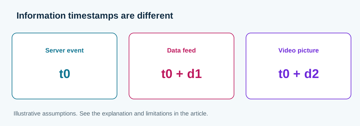
YouTube documents different latency modes and buffering trade-offs. Those platform settings do not measure the whole path from a tournament server through production to a viewer. A local stopwatch, a game clock and a provider timestamp are not interchangeable. Compare an identifiable event before subtracting times, and mark the gap unknown when the reference is missing.
For a constructed example, suppose the event reaches a pricing service after 0.52 seconds and the viewer after 55 seconds. The difference is 54.48 seconds, and the ratio is about 105.77. These are chosen inputs, not provider benchmarks. The ratio does not determine how many kills occurred, whether a round ended, or whether the offered selection has already settled. That would require further evidence about the event and market.
Accepted requests are a selected sample
A pending request, a rejection, a revised quote and an accepted wager are separate statuses. An animation does not reveal which rule produced them. To illustrate possible selection bias, suppose the probability changes to either 0.60 or 0.40, each with chance 0.50. Assign acceptance probabilities of 0.25 and 0.75 respectively. These are invented probabilities; no claim is made that a bookmaker uses this rule.
P(H) = P(L) = 0.50
p(win | H) = 0.60; p(win | L) = 0.40
P(accepted | H) = 0.25; P(accepted | L) = 0.75
p(win | H, accepted) = 0.60; p(win | L, accepted) = 0.40
P(accepted) = 0.50 × 0.25 + 0.50 × 0.75 = 0.50
p(win | accepted) = (0.50 × 0.25 × 0.60 + 0.50 × 0.75 × 0.40) / 0.50
                  = 0.45
EV/accepted = 0.45 × 1.95 - 1 = -0.1225 = -12.25%
EV/request = 0.50 × -0.1225 = -0.06125
At odds 1.95, the selected sample has EV -12.25% per accepted unit. Counting rejected requests as losing one-unit bets would be another mistake: under the example's no-fee assumption, they have no wager result. Per request, the expected net is 0.50 × -0.1225 = -0.06125 units. The denominator matters when comparing an execution process with a record of accepted tickets.
If both states instead have acceptance probability 0.50, the overall acceptance rate remains 0.50, but the conditional win probability becomes 0.50 and EV becomes -2.5%. The same acceptance rate therefore supports different returns. Establishing real asymmetric acceptance needs all requests and contemporaneous information, not only losing tickets or the results that happened after rejected requests.
Do not pay the margin twice in the calculation
For decimal odds O and a defensible probability p, net expectation per unit is p × O - 1. The offered price already contains its pricing disadvantage. Do not subtract a market's overround again from that EV. De-vig methods estimate a reference probability under additional assumptions; none turns a price into a known true chance. The odds converter checks the arithmetic, not the quality of the forecast.
A later reference also needs a comparable state. The line at the next freeze time may include another completed round, different cash and new information. Calling its difference from your price live CLV does not remove those changes. Define the comparison rule and preserve both states. A favorable subsequent move alone is not proof that the original forecast was correct.
A series calculation still needs the remaining maps
Consider independent maps with the same assumed win probability 0.60. Before a Bo3, winning at least two maps has probability 0.648. After a confirmed 1-0 lead, the probability of winning the series is 0.84 if the two remaining map probabilities are still 0.60 under the model. At a hypothetical quote 1.25, that gives +5% EV. It is a conditional calculation, not an observed pricing error.
p = 0.60
P(Bo3) = p²(3 - 2p) = 0.648
P(series | 1-0) = p + (1-p)p = 0.84
EV(1.25) = 0.84 × 1.25 - 1 = +5%
p2 = 0.55; p3_given_loss2 = 0.65
P(series | 1-0) = 0.55 + 0.45 × 0.65 = 0.8425
Both remaining maps matter. With second-map probability 0.55 and conditional decider probability 0.65 after losing map two, the result is 0.55 + 0.45 × 0.65 = 0.8425. You cannot get either result from the 1-0 score alone. Update the roster, veto and assumptions before reusing a pre-match estimate; the first map may itself contain information that changes them.
For a round-state model, use V(s) = q(s)V(s after win) + (1-q(s))V(s after loss), with the state containing the relevant score, side, cash and rules. Economy changes on both branches. Terminal conditions must match regulation and overtime rather than treating every thirteen-round score as the same event. A recursion written on paper does not validate the transition probabilities.
Exact tails can differ from a rough normal approximation
Suppose a hypothetical game has 30 recorded kills and the total line is Over 52.5. The event needs at least 23 additional kills. Assume a fixed remaining interval with mean 16.5. Compare Poisson with a negative binomial model of the same mean and shape r=8. No match dataset is supplied to justify the mean, remaining duration or shape; they are deliberately assumed inputs.
X = additional kills; X >= 23
mu = 16.5; r = 8; theta = r/(r+mu) = 16/49
Poisson: P(X=k) = exp(-16.5) × 16.5^k / k!
NB: P(X=k) = C(k+7,7) × (16/49)^8 × (33/49)^k
P(X>=23) = 1 - sum(P(X=k), k=0..22)
Poisson tail = 7.521873%
NB variance = 16.5 + 16.5²/8 = 50.53125
NB tail = 18.704806%
EV(Poisson, 9.00) = -32.303145%
EV(NB, 9.00) = +68.343258%
The definitions are documented by SciPy for Poisson and negative binomial. The tail values here were calculated by summing discrete probabilities, not treating a normal approximation as exact. At hypothetical odds 9.00, the corresponding EV values are -32.303145% and +68.343258%.
The sign changes because the probability model changes. That does not establish which model fits real kills, how long the game will last or whether the quote is available. A wider variance need not increase every possible tail probability at every threshold. Estimate and validate the distribution on comparable data before interpreting the calculation as a forecast; do not choose r after seeing which value produces a positive EV.
Keep an auditable forecast rather than a speed story
Save the event and market identifiers, information source, observed score, local time, model version and quote. Keep submission and final response separately, including rejected and changed requests. A paper simulation can test this record without placing bets. Preserve the original probability when later information requires a revision, so the old and new decisions can be distinguished.
The Live match-state probability model (EsportsMath) gives further modeling context, not independent verification of an observed edge here. The market-selection guide and timeout guide address related questions. A timeout, a familiar map or an apparent scaling advantage is an input to examine, never a substitute for a current state, supported probability and accepted price.